Interpolation

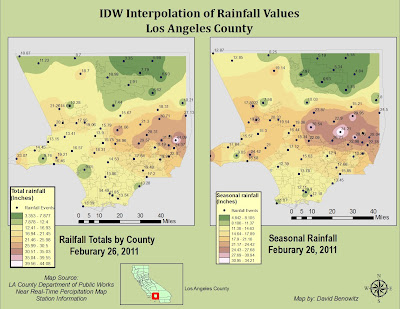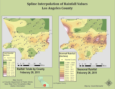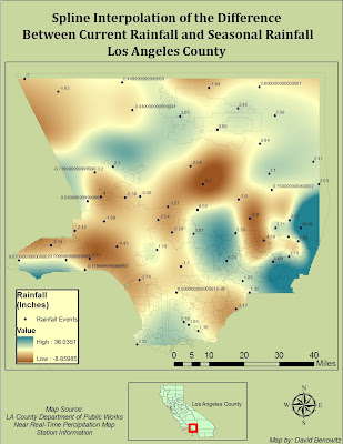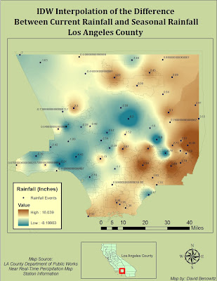
I started out the assignment by converting the degrees, minutes, and seconds of the location of each “Rain Sensor” to decimal degrees and determined the difference between seasonal Normal Rainfall and Current Total precipitations in Los Angeles County. I converted the Excel file to a database frame and projected the .dbf as XY data onto the polygon of Los Angeles County, both in the NA 1983 Datum Geographic Coordinate System. I then used spatial analyst to create Spline and IDW models of the Total and Normal interpolations, as well as the differences between them two especial in the San Gabriel Mountains in the North of LA County.

The interpolation of the rainfall of Los Angeles County are both revealing and intriguing. These rainfall patterns are show that the rainfall is pretty evenly distributed across LA County with one area of concentration of strong rainfall is the East, and weak rainfall in the North. The map showing the differences between the Total Rainfall and the Normal Rainfall shows that there are discrepancies between the two. There are also differences between the two that can clearly be seen in the maps.

I chose IDW and Spline interpolations because they are more accurate than Kriging on the local scale. They are also both efficient at estimating unknown points, which I felt was useful because I only used about 60 of the counties to build my interpolation. Because rainfall is so precisely tied to proximity in terms of regions, I felt IDW would be an accurate representation as well due to its function of interpolating points based on its distance Values. Spline interpolation has the ability to calculate exact surfaces for continuous temperature data which I felt helped in appropriately showing continuous rainfall throughout the county.